align_dates_seasonal() standardizes dates from multiple years to enable comparison of epidemic curves
and visualization of seasonal patterns in infectious disease surveillance data.
Commonly used for creating periodicity plots of respiratory diseases like
influenza, RSV, or COVID-19.align_and_bin_dates_seasonal() is a convenience wrapper that first aligns the dates and then bins the data to calculate counts and incidence.
Usage
align_dates_seasonal(
  x,
  dates_from = NULL,
  date_resolution = c("week", "isoweek", "epiweek", "day", "month"),
  start = NULL,
  target_year = NULL,
  drop_leap_week = TRUE
)

align_and_bin_dates_seasonal(
  x,
  dates_from,
  n = 1,
  population = 1,
  fill_gaps = FALSE,
  date_resolution = c("week", "isoweek", "epiweek", "day", "month"),
  start = NULL,
  target_year = NULL,
  drop_leap_week = TRUE,
  .groups = "drop"
)
Arguments
- x
Either a data frame with a date column, or a date vector.
Supported date formats aredateanddatetimeand also commonly used character strings:ISO dates
"2024-03-09"Month
"2024-03"Week
"2024-W09"or"2024-W09-1"
- dates_from
Column name containing the dates to align and bin. Used when x is a data.frame.
- date_resolution
Character string specifying the temporal resolution. One of:
"week"or"isoweek"- Calendar weeks (ISO 8601), epidemiological reporting weeks as used by the ECDC."epiweek"- Epidemiological weeks as defined by the US CDC (weeks start on Sunday)."month"- Calendar months"day"- Daily resolution
- start
Numeric value indicating epidemic season start, i.e. the start and end of the new year interval:
For
week/epiweek: week number (default: 28, approximately July)For
month: month number (default: 7 for July)For
day: day of year (default: 150, approximately June) If start is set to "1" the alignment is done for yearly comparison and the shift in dates for seasonality is skipped.
- target_year
Numeric value for the reference year to align dates to. The default target year is the start of the most recent season in the data. This way the most recent dates stay unchanged.
- drop_leap_week
If
TRUEand date_resolution isweek,isoweekorepiweek, leap weeks (week 53) are dropped if they are not in the most recent season. Set toFALSEto retain leap weeks from all seasons. Dropping week 53 from historical data is the most common approach. Otherwise historical data for week 53 would map to week 52 if the target season has no leap week, resulting in a doubling of the case counts.- n
Numeric column with case counts (or weights). Supports quoted and unquoted column names.
- population
A number or a numeric column with the population size. Used to calculate the incidence.
- fill_gaps
Logical; If
TRUE, gaps in the time series will be filled with 0 cases. Useful for ensuring complete time series without missing periods. Defaults toFALSE.- .groups
See
dplyr::summarise().
Value
A data frame with standardized date columns:
year: Calendar year from original dateweek/month/day: Time unit based on chosen resolutiondate_aligned: Date standardized to target yearseason: Epidemic season identifier (e.g., "2023/24"), ifstart = 1this is the year only (e.g. 2023).current_season: Logical flag for most recent season
Binning also creates the columns:
n: Sum of cases in binincidence: Incidence calculated using n/population
Details
This function helps create standardized epidemic curves by aligning surveillance data from different years. This enables:
Comparison of disease patterns across multiple seasons
Identification of typical seasonal trends
Detection of unusual disease activity
Assessment of current season against historical patterns
The alignment can be done at different temporal resolutions (daily, weekly, monthly) with customizable season start points to match different disease patterns or surveillance protocols.
Examples
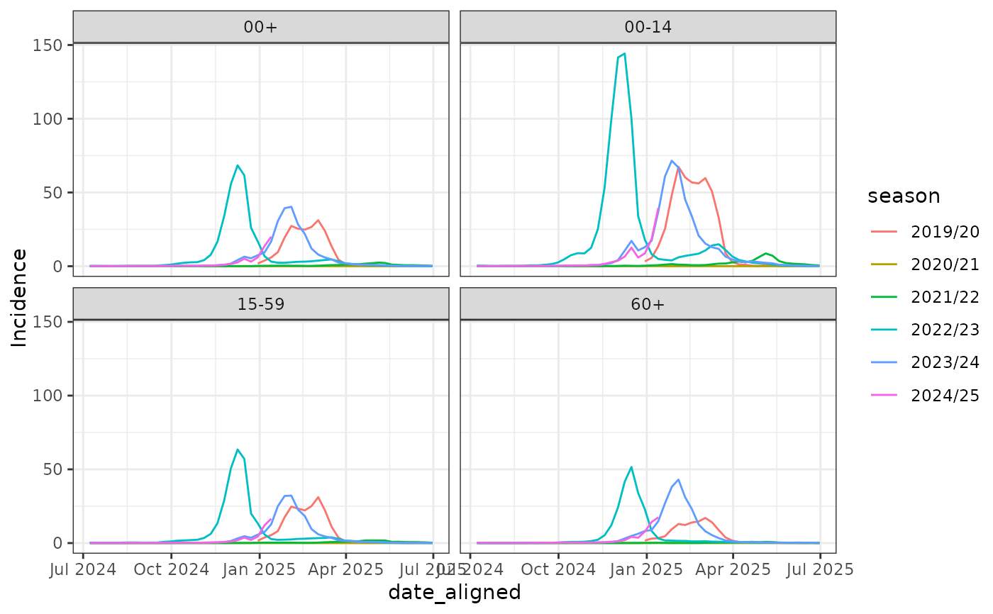
# Seasonal Visualization of Germany Influenza Surveillance Data
library(ggplot2)

influenza_germany |>
  align_dates_seasonal(
    dates_from = ReportingWeek, date_resolution = "epiweek", start = 28
  ) -> df_flu_aligned

ggplot(df_flu_aligned, aes(x = date_aligned, y = Incidence, color = season)) +
  geom_line() +
  facet_wrap(~AgeGroup) +
  theme_bw() +
  theme_mod_rotate_x_axis_labels_45()